Analysis of Prevalence of Mental Illnesses and Suicide in Different Countries Using Gower Clustering Based Dimensionality Reduction of Growth Metrics and Simulation-Based Hypothesis Testing

Source code for this research: https://github.com/AnilBattalahalli/Analysis-Of-Mental-Illnesses

Introduction

In the last two decades, there have been significant developments in understanding the anatomy of the brain for mental illnesses like Major Depressive Disorder, Anxiety Disorder, Bipolar Disorder, Schizophrenia, Personality Disorder, etc. Most of these disorders, along with alcohol and drug abuse are studied together to analyze the possible coexistence and the quantification of the correlation. One such study by Muester, et. al^[1], estimates high rates of co-occurring mental illnesses and substance use disorders at around 50%. While studying the psychiatric and pharmacological aspects of such disorders is very important for treating, studying the environmental and genetic predispositions of a mental illness can help regulate and mitigate its effect at an early stage.

Even though it’s estimated that 10% of the world population suffers from some psychiatric illness, as pointed out by WHO, one of the most common barriers for the countries to provide healthcare to the citizens with mental health disorders is the cultural and social stigma against mental illnesses. In addition to this, there are problems concerning lack of education, limited availability of mental health professionals, and limited affordability (poverty)^[2]. Also, systematic repression, starvation, human rights abuse can contribute to mental illnesses like PTSD, anxiety, and depression, as pointed out in a study by Riadh T. Abed^[3].

Studies involving socio-economic triggers like income, history of abuse, genetic history, employment status, etc can never be causal, as the random assignments of the test subjects to study the causation of the aforementioned parameters are unethical^[4]. Instead, the associative studies for the same can give us valuable insights regarding the parameters involved.

In this research, I analyze the association of schizophrenia, depression, anxiety, bipolar disorder, alcohol abuse, drug abuse, and suicide, with the GDP per capita, Human Development Index (HDI), unemployment rate, and population. The analysis employs clustering to stratify the samples into developed and underdeveloped countries. 

The illness rates are then compared with bootstrapped hypothesis tests and the inferences are thus drawn. The following report contains five sections: Data, Methodology, Simulation, Analysis, and Discussion.

Data

The dataset regarding the prevalence of mental illnesses was obtained by the Institute for Health Metrics and Evaluation^[5] which contains the percentage of people in a country suffering from a particular mental illness from 1990 to 2017. I also obtained multiple Human Development Report records from the United Nations Development Programme^[6] containing GDP per capita, population, suicide rate, unemployment rate, and Human Development Index (HDI) for different countries from 1991 to 2017. These records were merged using pandas for python by handling exceptions and missing values. The data was then cleaned up to avoid redundancies and rows with missing values were eliminated.

In addition to these, I added a few ‘flag’ variables that can be used for manual stratification for further analysis. The basis for the stratification is to differentiate developed and underdeveloped countries, to analyze the mental health landscape in a paired fashion. These flags are boolean features that are obtained by implementing a cutoff for the variables HDI, GDP Per capita, and Unemployment Rates. Along with the same, we also cut off the year in which the data was recorded. The cutoff value of 2010 was chosen for the same as 90% of the countries in the world had access to the internet connection. This would serve as an indicator to see if the development of technology impacts the variables of interest. Similarly, a cutoff of 6% for the unemployment rate and $3,000^[7] for GDP per capita was chosen.

library("GGally")
library(ggplot2)
library(dplyr)
library(boot)
library(gridExtra)
library(parallel)
library(vegan)
library(cluster)
library(coin)
options(warn=-1)
set.seed(84884)

cl <- makeCluster(detectCores())
df <- read.csv('absolute_grand_final.csv')
df$unef <- ifelse(df$unemp <= 6, TRUE, FALSE)
df$hdif <- ifelse(df$HDI >= 0.55, TRUE, FALSE)
df$intf <- ifelse(df$Year >= 2010, TRUE, FALSE)
df$gdppcf <- ifelse(df$GDP >=3000, TRUE, FALSE)

The dataset thus obtained has 17 variables and 3749 observations. The curated list of variables are as follows:

1. Name of the Country (Country)
2. Year of recording (Year)
3. Percentage of the population with Schizophrenia (schiz_perc)
4. Percentage of the population with Bipolar Disorder (bipolar _perc)
5. Percentage of the population with Anxiety (anxiety_perc)
6. Percentage of the population with Depression (depr_perc)
7. Percentage of the population with Drug Abuse (drug_perc)
8. Percentage of the population with Alcohol Abuse (alc_perc)
9. Unemployment rate (unemp)
10. Number of suicide per 100,000 people (suicide_tt)
11. The population of the country (pop)
12. GDP per capita of the country (GDP)
13. Human Development Index (HDI)
14. Flag for unemployment. (>6 is recorded as underdeveloped) (unef)
15. Flag for HDI. (<0.55 is recorded as underdeveloped) (hdif)
16. Flag for the internet. (<2010 is recorded as underdeveloped) (intf)
17. Flag for GDP (< 3000 is considered as underdeveloped) (gdppcf)

For inspection, we can plot the correlation plot between the numerical variables. The method uses Pearson’s correlation method internally. Since this is not stratified, the global inference for correlation may suffer a high bias^[8].

df_num <- subset(df, select = -c(Country, unef, hdif, intf, gdppcf))
ggcorr(
  df_num,
  geom = "tile",
  max_size = 6,
  size = 3.5,
  hjust = 0.75,
  #angle = -45, 
  color = "grey50",
  label = TRUE,
  label_size = 3, 
  label_round = 2, 
  label_alpha = TRUE,
  palette = ""
)

To see if our manual stratification method shows any significant boundary between the developed and underdeveloped countries, we can plot densities using the stratification flag as a label. If we use the GDP flag to check the growth metrics of a country, we get the following plot.

a <- ggplot(df, aes(x = HDI, color = hdif, fill = hdif)) + geom_density(alpha = 0.5)+theme_minimal()+xlab("HDI")
b <- ggplot(df, aes(x = GDP, color = hdif, fill = hdif)) + geom_density(alpha = 0.5)+xlim(c(0, 20000))+xlab("GDP Per Capita")+theme_minimal()
c <- ggplot(df, aes(x = pop, color = hdif, fill = hdif)) + geom_density(alpha = 0.5)+xlim(c(0, 1000000))+xlab("Population")+theme_minimal()
d <- ggplot(df, aes(x = unemp, color = hdif, fill = hdif)) + geom_density(alpha = 0.5)+xlab("Unemployment Rate")+theme_minimal()
grid.arrange(a, b, c, d, nrow=2, ncol=2)

Methodology

My first aim is to find out if the mental illnesses rates are mutually independent of one another. For example, mental illnesses like bipolar disorder and anxiety disorders are found to be highly correlated^[9]. Before we employ a method to compare independence, we need to see if the data follows a normal distribution. 

a <- ggplot(df, aes(x = bipolar_perc)) + geom_density(alpha = 0.5)+theme_minimal()+xlab("Bipolar Disorder")+ylab("Density")
b <- ggplot(df, aes(x = anxiety_perc)) + geom_density(alpha = 0.5)+xlab("Anxiety")+ylab("Density")+theme_minimal()
c <- ggplot(df, aes(x = schiz_perc)) + geom_density(alpha = 0.5)+xlab("Schizophrenia")+ylab("Density")+theme_minimal()
d <- ggplot(df, aes(x = depr_perc)) + geom_density(alpha = 0.5)+xlab("Depression")+ylab("Density")+theme_minimal()
grid.arrange(a, b, c, d, nrow=2, ncol=2)

The data looks like it deviates from the normal distribution quite a bit. To quantify the normality, we can use the Shapiro-Wilk test, with the test statistic given by,

where x(i) is the order statistic and x is the mean of the sample.

dis <- c("schiz_perc", "bipolar_perc", "anxiety_perc", "depr_perc")
c <- t(combn(dis,2))

for (i in dis){
  shapiro.test(as.numeric(unlist(df[i])))
}

The Shapiro-Wilk tests evaluated on all of the illnesses have the p-value < 2.2e-16. This implies that we reject the hypothesis that the variables are normally distributed. Since we know that the variables are not normally distributed, we can use a non-parametric, distribution-free test for independence like a permutation test. 

In this research, I have employed a two-sided permutation test for independence, and we can also quantify the association by bootstrapped analysis of the correlation. Here, I use the Pearson’s correlation given by,

The corresponding hypothesis test is given by,

The second aim of the research is to analyze the mean difference in the rate of mental illnesses between the developed and underdeveloped countries. Now the criteria for classifying the countries into developed and underdeveloped are not well defined. According to the United Nations’ M49 standards for classification^[14][15], “The designations “developed” and “developing” are intended for statistical convenience and do not necessarily express a judgment about the stage reached by a particular country or area in the development process.”

To analyze the effect of a country on the prevalence of a mental illness, we can differentiate the developed countries from underdeveloped countries concerning a cutoff like GDP Per Capita and then analyze the paired mean tests. But in doing so, we would be ignoring the other metrics which may contain useful information for the cut-off. We need a better way of clustering the variables^[10]. 

In this research, I employ two methods for the stratification of the countries into the aforementioned classes:

1. HDI based stratification
2. Clustering-based stratification

In the HDI-based stratification, we employ a cut-off value for the HDI, and we classify the countries into one of the two classes depending on their HDI being higher or lower than the cutoff. In the clustering-based stratification, we use clustering methods for all the growth parameters, and we interpret the clusters qualitatively to see if they form a well-defined boundary concerning the individual growth parameters.

In the research by Elizabeth Tipton^[11], the method discussed employs dividing the population samples into strata using unsupervised clustering for estimating boundary conditions concerning multiple variables. One of the proposed methods employs k-means clusters to stratify the samples. As opposed to euclidean distance, which is commonly used for the k-means clustering, we use the Gower distance metric. This is a general coefficient of similarity, which was proposed by Gower^[12] in 1971, given by,

For the two methods of stratification, I perform the bootstrap simulations to test for the difference in means for each mental illness and suicide rate. For each simulation, I generate the 95% confidence interval to test the hypothesis. If the interval at 95% confidence contains the null value (0), I do not reject the null hypothesis.

Simulations

In this research, I implement the two-sided permutation test for independence with 10000 Monte-Carlo samples and approximate density estimation.

dis <- c("schiz_perc", "bipolar_perc", "anxiety_perc", "depr_perc")
c <- t(combn(dis,2))

for (i in 1:dim(c)[1]){
  print(independence_test(as.formula(paste(c[i,1], '~' , c[i,2])), df, distribution = approximate(10000)))
}

The results are as follows:

	Schizophrenia	Bipolar Disorder	Anxiety Disorder	Depression
Schizophrenia	–	< 1e-04	< 1e-04	< 1e-04
Bipolar Disorder	< 1e-04	–	< 1e-04	< 1e-04
Anxiety Disorder	< 1e-04	< 1e-04	–	< 1e-04
Depression	< 1e-04	< 1e-04	< 1e-04	–

This shows that we can reject the null hypothesis that the variables are independent. The problem boils down to finding the 95% confidence interval for the correlation coefficient to see if it contains 0, which is the null value. As mentioned before, we use bootstrapping with 1000 bootstrap replications. Bootstrapping is implemented with parallelization for the effective utilization of the CPU cycles. If we use bootstrapping for every pair of mental illnesses and suicide rates, we get the following confidence intervals.

get_corr <- function(x, index){
  a = names(x)[1]
  b = names(x)[2]
  x_sample <- x[index,]
  return(cor(x_sample[a],x_sample[b]))
}

do_boot <- function(x){
  print(names(x))
  boot_corr <- boot(x, statistic = get_corr, R = 1000, parallel = 'snow', cl=cl)
  print(boot.ci(boot_corr, type = c("basic"), conf = 0.95))
  cat("\n\n")
}

for (i in 1:dim(c)[1]){
  do_boot(df[c[i,]])
}

	Schizophrenia	Bipolar Disorder	Anxiety Disorder	Depression	Suicide
Schizophrenia	1	(0.3392,0.4170)	(0.4686,0.5265)	(0.0657,0.1354)	(-0.1433, -0.1025)
Bipolar Disorder	(0.3392,0.4170)	1	(0.6775,0.7106)	(0.1433,0.2009)	(-0.2320, -0.1834)
Anxiety Disorder	(0.4686,0.5265)	(0.6775,0.7106)	1	(0.2911,0.3418)	(-0.2036, -0.1571)
Depression	(0.0657,0.1354)	(0.1433,0.2009)	(0.2911,0.3418)	1	(0.3294,0.3828)
Suicide	(-0.1433, -0.1025)	(-0.2320, -0.1834)	(-0.2036, -0.1571)	(0.3294,0.3828)	1

While we see that mental illnesses are mutually positively correlated, we can also see that illnesses like bipolar disorder, schizophrenia, and anxiety disorders are strongly negatively correlated with the suicide rate. Furthermore, all the variables are mutually correlated to each other, hence we reject the hypothesis that the variables are uncorrelated. When the same test for correlation is repeated for the growth metrics, we get the following confidence intervals.

dis <- c("pop", "GDP", "HDI")
c <- t(combn(dis,2))

get_corr <- function(x, index){
  a = names(x)[1]
  b = names(x)[2]
  x_sample <- x[index,]
  return(cor(x_sample[a],x_sample[b]))
}

do_boot <- function(x){
  print(names(x))
  boot_corr <- boot(x, statistic = get_corr, R = 1000, parallel = 'snow', cl=cl)
  print(boot.ci(boot_corr, type = c("basic"), conf = 0.95))
  cat("\n\n")
}

for (i in 1:dim(c)[1]){
  do_boot(df[c[i,]])
}

	Population	HDI	GDP Per Capita
Population	1	(-0.0573, -0.0214)	(-0.0921, -0.0700)
HDI	(-0.0573, -0.0214)	1	( 0.6749, 0.7057)
GDP Per Capita	(-0.0921, -0.0700)	( 0.6749, 0.7057)	1

The simulation result shows that the population is negatively correlated with HDI and GDP Per Capita. HDI and GDP Per Capita are positively correlated. We reject the null for the same aforementioned reasons. Now for the difference in mean hypothesis, as mentioned before, I use two methods of stratification. Firstly for the HDI-based stratification, I employed the flags that I set previously. We can plot the strata for the year 2000 to understand the clustering.

valcol <- c("schiz_perc","bipolar_perc","anxiety_perc","drug_perc","depr_perc","alc_perc","suicide_tt")

ggplot(df[df$Year == 2000,], aes(GDP,HDI,color=hdif)) + geom_point(size = 0.1, stroke = 0, shape = 16) + geom_text(aes(label=Country), size=3)+theme_minimal()

We can plot the density for the illnesses and the growth parameters based on this criterion.

a <- ggplot(df, aes(x = HDI, color = strata, fill = strata)) + geom_density(alpha = 0.5)+theme_classic()
b <- ggplot(df, aes(x = GDP, color = strata, fill = strata)) + geom_density(alpha = 0.5)+xlim(c(0, 20000))+theme_classic()
c <- ggplot(df, aes(x = pop, color = strata, fill = strata)) + geom_density(alpha = 0.5)+theme_classic()+xlim(c(0, 1000000))
d <- ggplot(df, aes(x = unemp, color = strata, fill = strata)) + geom_density(alpha = 0.5)+theme_classic()
grid.arrange(a, b, c, d, nrow=2, ncol=2)

a <- ggplot(df, aes(x = bipolar_perc, color = hdif, fill = hdif)) + geom_density(alpha = 0.5)+theme_classic()
b <- ggplot(df, aes(x = schiz_perc, color = hdif, fill = hdif)) + geom_density(alpha = 0.5)+theme_classic()
c <- ggplot(df, aes(x = anxiety_perc, color = hdif, fill = hdif)) + geom_density(alpha = 0.5)+theme_classic()
d <- ggplot(df, aes(x = depr_perc, color = hdif, fill = hdif)) + geom_density(alpha = 0.5)+theme_classic()
grid.arrange(a, b, c, d, nrow=2, ncol=2)

ggplot(df, aes(x = suicide_tt, fill = hdif)) + geom_density(alpha = 0.5)+theme_classic()

Now we perform clustering-based stratification. The growth metrics, along with the flags are used as inputs for clustering. The numerical values are normalized to satisfy the equal variance condition required by the k-means algorithm. Gower metric works for both categorical and numerical variables^[13] and hence my binary flag variables don’t have to be numerical and scaled. We can plot the strata for the year 2000 to understand the clustering.

u <- df %>% select(c("Year","GDP","HDI","unef","hdif","intf","gdppcf","pop")) %>% 
      mutate_if(is.numeric, scale) %>% 
      vegdist(method = "gower") %>% 
      pam(k=2, diss=TRUE) 

df$strata <- ifelse(u$clustering == 1, yes=TRUE, no=FALSE)

ggplot(df[df$Year == 2000,], aes(GDP,HDI,color=strata)) + geom_point(size = 0.1, stroke = 0, shape = 16) + geom_text(aes(label=Country), size=3)

Clustered variables are used as stratification labels and we can plot the densities of the growth metrics with the stratification label fills.

a <- ggplot(df, aes(x = HDI, color = strata, fill = strata)) + geom_density(alpha = 0.5)+theme_classic()
b <- ggplot(df, aes(x = GDP, color = strata, fill = strata)) + geom_density(alpha = 0.5)+xlim(c(0, 20000))+theme_classic()
c <- ggplot(df, aes(x = pop, color = strata, fill = strata)) + geom_density(alpha = 0.5)+theme_classic()+xlim(c(0, 1000000))
d <- ggplot(df, aes(x = unemp, color = strata, fill = strata)) + geom_density(alpha = 0.5)+theme_classic()
grid.arrange(a, b, c, d, nrow=2, ncol=2)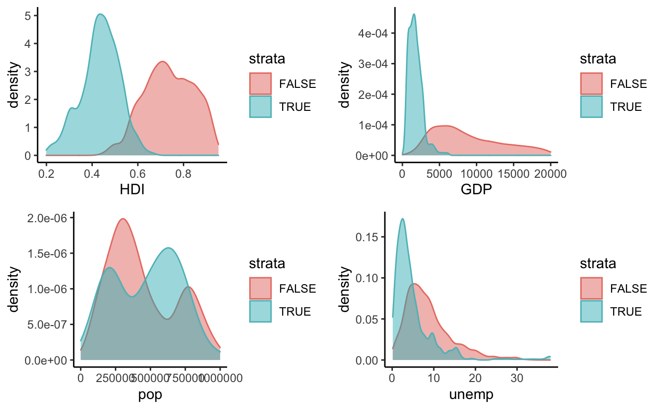

We can see that the red density curve represents higher GDP and higher HDI and hence, generally covers the developed countries. Now we can also plot the densities of the illness according to this strata.

The density plot shows some distinctions in the distributions of mental illnesses. To obtain quantified differences and the respective confidence intervals for the paired means, we can perform a simulation using bootstrapping. 

a <- ggplot(df, aes(x = bipolar_perc, color = strata, fill = strata)) + geom_density(alpha = 0.5)+theme_classic()
b <- ggplot(df, aes(x = schiz_perc, color = strata, fill = strata)) + geom_density(alpha = 0.5)+theme_classic()
c <- ggplot(df, aes(x = anxiety_perc, color = strata, fill = strata)) + geom_density(alpha = 0.5)+theme_classic()
d <- ggplot(df, aes(x = depr_perc, color = strata, fill = strata)) + geom_density(alpha = 0.5)+theme_classic()
grid.arrange(a, b, c, d, nrow=2, ncol=2)

We can see that the two clustering methods perform similarly. But, using a cluster that is representative of multiple variables seems to be more intuitive. Hence, I proceed with Gower clustering for bootstrapped hypothesis testing of paired means.

We use the statistic T = xu-xd where xu is the sample mean of the underdeveloped countries and xd is the sample mean of the developed countries. We perform bootstrapping with 1000 bootstrap replicates.

get_meandiff <- function(x, index, a){
  x_sample <- x[index,]
  return(mean(as.matrix(x_sample[!x_sample$strata,][a]))-mean(as.matrix(x_sample[x_sample$strata,][a])))
}

valcol <- c("schiz_perc","bipolar_perc","anxiety_perc","drug_perc","depr_perc","alc_perc","suicide_tt")

for (i in valcol){
  print(i)
  boot_corr <- boot(df, statistic = get_meandiff, a = i, R = 1000, parallel = 'snow', cl=cl)
  print(boot.ci(boot_corr, type = c("basic"), conf = 0.95))
  cat("\n\n")
}

The result of the bootstrap analysis with a 95% confidence interval for the difference of mean between the underdeveloped and the developed countries for the variables of interest are as follows:

Variable of Interest	Confidence Interval
Schizophrenia	( 0.0381,  0.0428 )
Bipolar Disorder	( 0.1572,  0.1721 )
Anxiety Disorder	( 0.8179,  0.9341 )
Depression	(-0.1927, -0.1093 )
Suicide	(-2.097, -1.166 )

Analysis

The outcome of the permutation test for independence suggests that the prevalence of mental illnesses suggests that there is evidence to show that the existence of mental illnesses is mutually correlated. This is pointed out in the research by Elliott, Marta, et al.^[16] which shows that there are many common explanatory factors for mental illnesses. In the quantification of the dependence using correlation, we obtain the following result at a 95% confidence interval.

	Schizophrenia	Bipolar Disorder	Anxiety Disorder	Depression	Suicide
Schizophrenia	1	(0.3392,0.4170)	(0.4686,0.5265)	(0.0657,0.1354)	(-0.1433, -0.1025)
Bipolar Disorder	(0.3392,0.4170)	1	(0.6775,0.7106)	(0.1433,0.2009)	(-0.2320, -0.1834)
Anxiety Disorder	(0.4686,0.5265)	(0.6775,0.7106)	1	(0.2911,0.3418)	(-0.2036, -0.1571)
Depression	(0.0657,0.1354)	(0.1433,0.2009)	(0.2911,0.3418)	1	(0.3294,0.3828)
Suicide	(-0.1433, -0.1025)	(-0.2320, -0.1834)	(-0.2036, -0.1571)	(0.3294,0.3828)	1

While it’s evident that mental illnesses are mutually positively correlated, Bipolar Disorder, Anxiety Disorders, and Schizophrenia seem to be negatively correlated with suicide. This is contradictory to the study by Novick, Danielle M, et al.^[17] which suggests that around  32.4% of the population with Bipolar II and 36.3% of the population with Bipolar I attempt suicide and between 4% and 19% of the people suffering from the illness complete suicide. A similar study estimates a rate of 4.9% for schizophrenia^[18] and 3.4% for anxiety disorders^[19]. 

In fact, a study by Arsenault-Lapierre, Geneviève et al.^[20] suggests that 90% of the deaths by suicide have had a history of mental illness. In my analysis, I have a strong negative correlation between mental illnesses and suicide rates which contradicts the previous studies.

Coming to the hypothesis testing for the difference in paired means ( u-d) of the mental illnesses and the suicide rates results in the following confidence intervals:

Variable of Interest	Confidence Interval
Schizophrenia	( 0.0381,  0.0428 )
Bipolar Disorder	( 0.1572,  0.1721 )
Anxiety Disorder	( 0.8179,  0.9341 )
Depression	(-0.1927, -0.1093 )
Suicide	(-2.097, -1.166 )

This implies that, for mental illnesses like Schizophrenia, Bipolar Disorder, and Anxiety disorder, the difference between the average population suffering from illnesses in underdeveloped countries with the ones in developed countries is positive. 

In other words, the percentage of the population suffering from these illnesses is greater in the developed countries. But, the rates of depression and suicide are higher in underdeveloped countries. We need to analyze this disparity further.

In the research by Kopinak, et al.^[21], the problems that the developing and underdeveloped countries face in the mental health sector on diagnosis, treatment, affordability, and education are discussed. In addition to this, it’s found that in many countries, Diagnostic Statistical Manual (DSM) which provides guidelines for mental illnesses is considered flawed which results in the under-diagnosis of the illnesses. When it comes to depression disorders, most of them are diagnosed by a primary care physician^[22]. Disorders like schizophrenia, bipolar disorder, anxiety disorders, personality disorders, etc are diagnosed by a specialist (typically a psychiatrist). Hence, the poor diagnosis and an inaccurate representation of the proportion of people suffering from these disorders can be attributed to the lack of availability, development, and research in the mental health landscape in those countries. 

While there are strict guidelines to report suicide to the United Nations by its member countries^[23], the same does not exist for mental illnesses as the diagnosis requires human resources specializing in the same^[24]. It’s estimated that in underdeveloped and developing countries, around 76% of people with mental illnesses receive no treatment for their disorder.

Discussion

In this literature, I have addressed the following research questions – 

1. Is there any evidence that the mental illness rates for different illnesses are correlated?
2. What is the mean difference in mental illnesses and suicide rates in developed and underdeveloped countries?

The data was obtained from Human Development Report records from the United Nations Development Programme. The data was cleaned up and variables of interest were retained and additional flag variables were created. To analyze the normality condition, the Shapiro-Wilk test was performed on each variable of the dataset. Following the non-normality of the dataset, a permutation test – a non-parametric distribution-free method was proposed to assess the independence of the variables (first research question). To assess the difference of paired means (second research question) the data were clustered to reduce the dimensionality of the growth factors followed by a bootstrap-based hypothesis testing.

In summary, we can attribute the lower percentages of mental illnesses like bipolar disorder, anxiety disorders, schizophrenia, etc, to the poor quality of data arising from the inadequate diagnostic systems. And more accurate data for suicides and depression owing to the feasibility in diagnosing and reporting in underdeveloped countries.

One of the assumptions made in the following analysis was that the samples are independent. But, the countries evolving over time can be considered a stochastic process and we need time-series methods for clustering the data. We can also employ hypothesis testing and parameter estimation for the time-series features to project the development of a country pertaining to the mental health landscape.

References

1. Drake, Robert E et al. “Management of persons with co-occurring severe mental illness and substance use disorder: program implications.” World psychiatry : official journal of the World Psychiatric Association (WPA) vol. 6,3 (2007): 131-6.
2. Kohrt, Brandon A et al. “The Role of Communities in Mental Health Care in Low- and Middle-Income Countries: A Meta-Review of Components and Competencies.” International journal of environmental research and public health vol. 15,6 1279. 16 Jun. 2018, doi:10.3390/ijerph15061279
3. Abed, Riadh T. “Tyranny and Mental Health.” British Medical Bulletin, vol. 72, no. 1, Oxford University Press (OUP), Jan. 2004, pp. 1–13. Crossref, doi:10.1093/bmb/ldh037.
4. Jain, Shobhit et al. “Ethics in Psychiatric Research: Issues and Recommendations.” Indian journal of psychological medicine vol. 39,5 (2017): 558-565. doi:10.4103/IJPSYM.IJPSYM_131_17
5. Global Burden of Disease Collaborative Network. Global Burden of Disease Study 2017 (GBD 2017) Results. Seattle, United States: Institute for Health Metrics and Evaluation (IHME), 2018.
6. HDRO calculations based on data from UNDESA (2019a), UNESCO Institute for Statistics (2020), United Nations Statistics Division (2020b), World Bank (2020a), Barro and Lee (2018) and IMF (2020)
7. World Bank, Constant GDP per capita for Low Income Countries [NYGDPPCAPKDLIC], retrieved from FRED, Federal Reserve Bank of St. Louis; https://fred.stlouisfed.org/series/NYGDPPCAPKDLIC, March 21, 2021.
8. Kaplan, Robert M et al. “Big data and large sample size: a cautionary note on the potential for bias.” Clinical and translational science vol. 7,4 (2014): 342-6. doi:10.1111/cts.12178
9. Simon, Naomi M et al. “Anxiety disorder comorbidity in bipolar disorder patients: data from the first 500 participants in the Systematic Treatment Enhancement Program for Bipolar Disorder (STEP-BD).” The American journal of psychiatry vol. 161,12 (2004): 2222-9. doi:10.1176/appi.ajp.161.12.2222
10. Elliott, Michael R. “A simple method to generate equal-sized homogenous strata or clusters for population-based sampling.” Annals of epidemiology vol. 21,4 (2011): 290-6. doi:10.1016/j.annepidem.2010.11.016
11. Tipton, Elizabeth. “Stratified Sampling Using Cluster Analysis: A Sample Selection Strategy for Improved Generalizations From Experiments.” Evaluation Review, vol. 37, no. 2, Apr. 2013, pp. 109–139, doi:10.1177/0193841X13516324.
12. Gower, J. C. “A General Coefficient of Similarity and Some of Its Properties.” Biometrics, vol. 27, no. 4, 1971, pp. 857–871. JSTOR, www.jstor.org/stable/2528823. Accessed 21 Mar. 2021.
13. Hummel, Manuela et al. “Clustering of samples and variables with mixed-type data.” PloS one vol. 12,11 e0188274. 28 Nov. 2017, doi:10.1371/journal.pone.0188274
14. “Standard Country and Area Codes Classifications (M49): Developed Regions”. United Nations Statistics Division. Archived from the original on 11 July 2017. Retrieved 13 May 2017.
15. “United Nations Statistics Division- Standard Country and Area Codes Classifications (M49)”. Unstats.un.org. Retrieved 15 January 2014.
16. Elliott, Marta, et al. “Subjective Accounts of the Causes of Mental Illness in the USA.” International Journal of Social Psychiatry, vol. 58, no. 6, Nov. 2012, pp. 562–567, doi:10.1177/0020764011415207.
17. Novick, Danielle M et al. “Suicide attempts in bipolar I and bipolar II disorder: a review and meta-analysis of the evidence.” Bipolar disorders vol. 12,1 (2010): 1-9. doi:10.1111/j.1399-5618.2009.00786.x
18. Hor, Kahyee, and Mark Taylor. “Suicide and schizophrenia: a systematic review of rates and risk factors.” Journal of psychopharmacology (Oxford, England) vol. 24,4 Suppl (2010): 81-90. doi:10.1177/1359786810385490
19. Nepon, Josh et al. “The relationship between anxiety disorders and suicide attempts: findings from the National Epidemiologic Survey on Alcohol and Related Conditions.” Depression and anxiety vol. 27,9 (2010): 791-8. doi:10.1002/da.20674
20. Arsenault-Lapierre, Geneviève et al. “Psychiatric diagnoses in 3275 suicides: a meta-analysis.” BMC psychiatry vol. 4 37. 4 Nov. 2004, doi:10.1186/1471-244X-4-37
21. Kopinak, Janice Katherine. “Mental Health in Developing Countries: Challenges and Opportunities in Introducing Western Mental Health System in Uganda.” International journal of MCH and AIDS vol. 3,1 (2015): 22-30.
22. Ng, Chung Wai Mark et al. “Major depression in primary care: making the diagnosis.” Singapore medical journal vol. 57,11 (2016): 591-597. doi:10.11622/smedj.2016174
23. “Suicide – Challenges and Obstacles.” World Health Organization, World Health Organization, www.who.int/news-room/fact-sheets/detail/suicide. 
24. Who.int. 2021. Mental disorders. [online] Available at: <https://www.who.int/news-room/fact-sheets/detail/mental-disorders> [Accessed 23 April 2021].