This project was co-authored by Heather Johnston and Youngwoo Kwon
$$ \newcommand{\boldphi}{\boldsymbol{\phi}} $$Introduction
COVID-19, or Coronavirus Disease 2019, was declared a pandemic by the World Health Organization on March 11, 2020. The disease originated in December 2019 in China and quickly spread around the world. Compared with the previous epidemics like Ebola and SARS, COVID-19 has a relatively low mortality rate, but spreads faster with numerous mildly symptomatic cases. In response to the spread of COVID-19, governments and institutions have implemented a variety of policies such as social distancing, masks requirements, stay-at-home orders, and travel restrictions to limit or prevent person-to-person interactions.
Our project explores the distribution of case numbers of COVID-19 in the United States over the past two years and how the infection and recovery rate have been changed during the pandemic. To determine how the shift between susceptible – inspection – recovery groups has occurred for coronavirus, our project adapts the conventional SIR model to estimate the infection and recovery rates using data reported at the daily level. The present project applies Monte Carlo Markov Chain to find the proposal distributions for infection rate and recovery rate, and the Metropolis-Hasting algorithm with prior distributions and proposal distributions to estimate the posterior distribution of infection rate and recovery rate. Eventually, the project forecasts the future pandemic data using infection rate and recovery rate from the previous data.
Data
The data for our project comes from the Oxford Government Responses Tracker, and the Our World in Data COVID-19 repository. The data from the Our World in Data Covid-19 data set includes infomration for each country each day with number of new cases and total population. The data from the Oxford Government Responses Tracker includes vaccination and facial covering policy for each location beginning in December of 2020, with results reported for users throughout much of the world.
The infection rate is an indicator of how probable it is that a susceptible person (ie a person who has never before been infected) will become infected in a given time period, which is subject to various factors such as government policy, the degree of infections of the virus in the country, or the degree of the mutation of the virus. To establish more accurate infection rates, our project filtered the data by choosing the United States as the location of interest. Our project set vaccination rate, mask policies, and degree of the mutation of the virus as the three main predictors with which to slice the data, allowing us to fit separate infection rates for each time period.
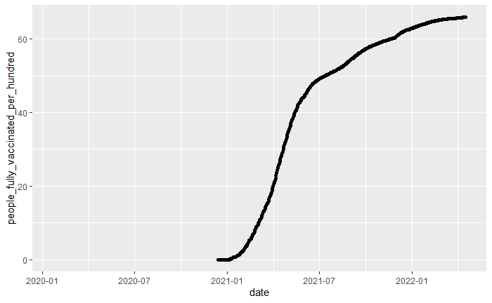
Figure 1. Fully vaccinated rate in United States from “2020-01-01” to “2022-04-10”
Figure 1 shows how the number of people fully vaccinated changed over time. A population with a higher fully-vaccinated percentage has a stronger resistance to viruses across the population, which results in a decrease in the infection rate. To reflect the strong relationship between the fully vaccinated rate and the infection rate, our project divided the data into two groups based on the time when the fully vacated rate reached $50\%$, which was July 13, 2021.
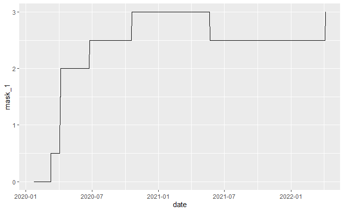
Figure 2. Facial Coverings policy in United States from “2020-01-01” to “2022-04-10”
Figure 2 shows how the mask policy in United States changed over time. A strong mask restriction policy can reduce the rate of virus transmission between people and consequently produce a low infection rate. Our project divided the data into three groups based on the time when the mask policy in United States have been changed from an average of 2.5 to 3, which is “2020-10-19” and “2021-05-23”.
On 26 November 2021, WHO designated a new variant of COVID-19, named Omicron. Compared to the original COVID-19 virus, Omicron spreads more quickly. Omicron resulted in a huge surge in cases in the pandemic around the world. Thus, our project divided the data into two parts, before and after the omicron, to reflect this impact, which is “2021-11-01”.
As a result, our research divided the time interval into five,
- Before “2020-10-19”
- From “2020-10-18” to “2021-05-23”
- From “2021-05-22” to “2021-07-13”
- From “2021-07-12” to “2021-11-01”
- From “2021-10-31” to “2022-04-10”
Methods
As discussed before, we use the SIR model to model the epidemic stochastic process. Even though the epidemic process is a continuous time stochastic process, we only observe the aggregated data for example: cases per day, cases per week, etc. Therefore, we need to make necessary adjustments to the model to describe the data.
Model
For the SIR model, we use three random variables to describe the epidemic process, $S(t)$, $I(t)$, and $R(t)$ where $S(t)$ is the number of infected people, $I(t)$ is the number of infected people, and $R(t)$ is the number of recovered people at time t. We can see that the random variables satisfy
$$ \begin{aligned} N &= S(t) + I(t) + R(t) \\ \frac{dN}{dt} &= \frac{dS(t)}{dt} + \frac{dI(t)}{dt} + \frac{dR(t)}{dt} \end{aligned} $$where N is the population of the system.
Between any two consecutive observations at $t_1$ and $t_2$ where $t_2-t_1 = \Delta t$, only one of the following three transitions can occur,
$(s, i) \xrightarrow{\Delta t} (s-1, i+1)$ corresponding to an infection event ($e_i$), $(s, i) \xrightarrow{\Delta t} (s, i-1)$ corresponding to a recovery event ($e_r$), or $(s, i) \xrightarrow{\Delta t} (s, i)$ corresponding to a null event ($e_n$). We can also write out the transition probabilities corresponding to the three events, where $s$ is the number of susceptible people and $i$ is the number of infected people in the population. It can be shown that,
where $\beta$ is the infection rate, and $\gamma$ is the recovery rate.
Therefore, the transition probabilities can be summarized as,
$$ \begin{align} p(\Delta t)=\begin{cases} \dfrac{\beta s i}{N} \Delta t, & \text{if} \ $(s, i) \xrightarrow{\Delta t} (s-1, i+1)$ \\ \gamma i \Delta t, & \text{if} \ $(s, i) \xrightarrow{\Delta t} (s, i-1)$ \\ 1 – \left[\dfrac{\beta s i}{N} \Delta t + \gamma i \Delta t \right], & \text{if} \ $(s, i) \xrightarrow{\Delta t} (s, i)$ \end{cases} \end{align} $$We can see that the transition probabilities change with each infection and recovery events which makes it challenging to deal with the daily aggregate epidemic data. To address this problem, we assume that the infection and recovery rates do not vary within each day.
We can now model the SIR infection process as,
$$ \begin{aligned} i_d &\sim \text{Poisson} \left(\frac{\beta \ S(t_{d}) \ I(t_{d})}{N} (t_{d} – t_{d-1})\right) \\ r_d &\sim \text{Poisson} \left(\gamma i (t_{d} – t_{d-1})\right) \end{aligned} $$where $i_d$ is the number of infection events on day $d$, $r_d$ is the number of recovery events on day $d$, $S(t_{d})$ is the number of susceptible people in the population at the beginning of day $d$, and $I(t_{d})$ is the number of infected people in the population at the beginning of day $d$. We model this as a Poisson random variable with constant arrival probabilities for within a day which helps us model the SIR model with aggregated infection and recovery count data.
The Bayesian framework
The Bayesian framework for the stochastic model can be written as follows,
$$ p(\phi \ | \ \mathcal{D}) \propto_{\phi} \mathcal{L}(\mathcal{D}, \phi) \ p(\phi) $$where,
$$ \mathcal{L}(\mathcal{D}, \phi) = \prod_{d \in D} p_{e_i}(i_d|i_{d-1}, \phi) \\ $$Now, the Bayesian framework for the estimation of the infection rate $\beta$ can be written as,
$$ \begin{align*} p(\beta \ | \ \mathcal{D}) &\propto_{\beta} \prod_{d \in D} p_{e_i}(i_d|i_{d-1}, \phi) \ p(\beta) \\ p(\beta \ | \ \mathcal{D}) &\propto_{\beta} \left[ \prod_{d \in D} \dfrac{\left(\dfrac{\beta S(t_d) I(t_d) \Delta t}{N}\right)^{i_d} \ \exp{\left\{- \dfrac{\beta S(t_d) I(t_d) \Delta t}{N}\right\}} }{i_d} \right] \ p(\beta) \\ \end{align*} $$We let $p(\beta)$ be a gamma prior as $\beta$ is always positive. We adjust the parameters such that, the mode of the distribution lies in the range $0.1 < \beta < 0.5$ based on previous studies.
Similarly, the Bayesian framework for the estimation of the recovery rate $\gamma$ can be written as,
$$ \begin{align*} p(\gamma \ | \ \mathcal{D}) &\propto_{\gamma} \prod_{d \in D} p_{e_i}(i_r|i_{d-1}, \phi) \ p(\gamma) \\ p(\gamma \ | \ \mathcal{D}) &\propto_{\gamma} \left[ \prod_{d \in D} \dfrac{\left(\gamma i \Delta t \right)^{i_r} \ \exp{\left\{- \gamma i \Delta t \right\}} }{i_r} \right] \ p(\gamma) \\ \end{align*} $$We let $p(\gamma)$ be a gamma prior again with appropriate parameters such that, the mode centers at the inverse of the average recovery period.
Simulation
To implement the Bayesian inference for the infection and rate parameters, we propose a data generative model followed by inference to check the efficacy of the algorithm. We adapated the data simulation method Kypraios et al. The data generation involves the following steps:
- Initialize $N$, $\beta$, $\gamma$, $s=N-1$, $i=1$, and $t=0$
- while $i > 0$ do,
- draw $\tau \sim \text{Exp}(\dfrac{\lambda}{N} s i + \gamma i)$
- draw $u \sim U(0,1)$
- if $u < \dfrac{\dfrac{\lambda}{N} s i }{\left(\dfrac{\lambda}{N} s i + \gamma i\right)}$, $s = s – 1$, $i = i + 1$, infectionFlag=1, removalFlag=0
- else, $i = i – 1$, infectionFlag=0, removalFlag=1
- $t = t + \tau$
- Record (s, i), (t), (infectionFlag, removalFlag)
- end while
Set $T_0$ such that $T_0$ corresponds to time duration with respect to $t$ in a day, and aggregate the simulated data to contain the following information.
- The day index $d$
- The total number of susceptible people in the population at the beginning of day $d$
- The total number of infected people in the population at the beginning of day $d$
- The total number of infection events on day $d$
- The total number of removal events on day $d$
Metropolis-Hasting algorithm
As discussed above, the likelihood function is a modification of the Poisson distribution and the prior distribution is a Gamma distribution. Since the posterior looks complex, we implement a simulation based method to draw inference. We use Metropolis-Hasting algorithm to draw from the posterior distribution.
The proposal distributions for $\beta$ and $\gamma$ are Log-Normal distributions with the mean centered around the interval $[0, 0.5]$ to steer the proposal sampler in the valid random walk path.
The proposal distributions are,
$$ \begin{aligned} \beta_{i} | \beta_{i-1} &\sim \text{lognorm}(ln(0.15)+1, \text{sigmoid}(1/\beta_{i-1})) \\ \gamma_{i} | \gamma_{i-1} &\sim \text{lognorm}(ln(0.1)+1, 1+ \text{sigmoid}(1/\gamma_{i-1})) \end{aligned} $$The Metropolis-Hasting algorithm can be implemented with the following steps
- Start with $\boldsymbol{\phi_0}$
- For $i=1, 2, \dots n$:
- Draw $\boldsymbol{\phi^+}$ from $q(\boldsymbol{\phi_{i-1}})$
- Compute $a = \frac{\mathcal{L}(\mathcal{D}, \boldsymbol{\phi^+}) q(\boldsymbol{\phi_{i-1}} | \boldsymbol{\phi^+})}{\mathcal{L}(\mathcal{D}, \boldsymbol{\phi_{i-1}}) q(\boldsymbol{\phi^+} | \boldsymbol{\phi_{i-1}})}$
- if $a > 1$, accept $\boldsymbol{\phi^+}$, $\boldsymbol{\phi_i} = \boldsymbol{\phi^+}$
- if $0 < a < 1$, accept $\boldsymbol{\phi^+}$, $\boldsymbol{\phi_i} = \boldsymbol{\phi^+}$ with probability $a$
Application
Utilizing data from the Our World in Data COVID-19 data repository, we consider the number of cases of COVID in the United States [Hannah Ritchie and Roser, 2020].
Since the pandemic has lasted more than two years, with numerous factors influencing the infection rate, such as social distancing, masking, vaccination, and variants, we choose to break the pandemic into five temporal sub-periods, based upon major events in the pandemic and the emergence of the Omicron variant. Furthermore, for the sake of simplicity, we assume that the only possible progression of states for an individual is from susceptible to infected to recovered. In other words, we assume negligible impact of waning immunity over time, and we assume that vaccinated people can still become infected.
Because recovery rates are unobserved (at least at the population level), we estimate recovery data in order to demonstrate the utility of our method. In order to estimate the recovery data, we implement a stochastic process using a log-linear model with parameters $\mu = 1.5$ and $\sigma^2 = .25$, where each new infection is assigned a value according to the log-linear model, and rounded to the nearest integer which is considered the number of days that person will take to recover. This model was chosen based on the CDC’s most recent guidance on infectious periods for COVID-19 [CDC 2020]. We assume that the recovery rate is the same throughout the pandemic. The chart below shows the observed number of new infections with vertical bars indicating the spaces in which we separate the periods to estimate the infection rate parameter.
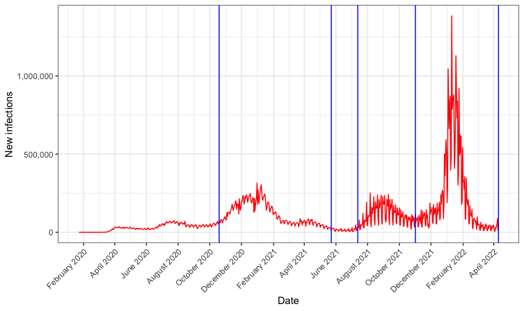
Figure 4: Observed numbers of new infections in the U.S. with vertical bars in blue indicating sub-period boundaries
The chart above shows our estimated rate of current infections, which depends both on the new infection rate (observed) and the recovery time of each individual (estimated). We also show with vertical lines the 4 dates separating the pandemic into 5 sub-periods for parameter estimation. In order to estimate these parameters, we set prior distributions for $\beta$ and $\gamma$ as follows:
$$ \begin{align*} p_0(\beta) & \sim \text{Gamma}(2, 5) \\ p_0(\gamma) & \sim \text{Gamma}(20, 95) \end{align*} $$We chose these distributions based on values estimated in previous papers for the infection and recovery rates for COVID-19 and earlier respiratory diseases like SARS, which tend to be between 0 and 1 [Wang et al., 2021, Wintachai and Prathom, 2021]. We allowed the proposal distributions to have a low probability of high values to allow for our uncertainty in the rates.
The proposal distributions for each new $\beta^+$ and $\gamma^+$ in the Markov Chain are as follows:
$$ \begin{align*} J_{\beta}(\beta^* | \beta_s) & \sim \text{Log-normal}(\mu = \log (0.2) + 1, \sigma = S(1/\beta_s)) \\ J_{\gamma}(\gamma^* | \gamma_s) & \sim \text{Log-normal}(\mu = \log (0.22) + 1, \sigma = 1+S(1/\gamma_s)) \end{align*}\ $$Where $S(.)$ denotes the sigmoid function, so $S(x) = [1 + e^{-x}]^{-1}$.
Forecasting U.S. case numbers
Utilizing the estimated infection rate $\beta$ and recovery rate $\gamma$ for the United States, we predict the data ranging from April 10, 2022 through April 30, 2022. We are able to assess the accuracy of our forecast for the eight days from April 10 through April 18 using visualization methods and numerical comparisons.
Results
After implementing our Metropolis-Hasting algorithm for estimating the parameters of the simulated infections data, we obtained a stable set of $\beta_s$ values representing our posterior distribution, with a posterior mean within rounding error of the true values for both parameters. We proceeded to apply our method to the actual U.S. COVID case data.
MCMC procedure diagnostics
When implementing our Metropolis-Hasting algorithm for the real COVID data, we witnessed that our algorithm converged quickly, with values not changing much after the initial accepted $\theta^+$. Furthermore, the acceptance rate for $\theta^+$ values generated from the proposal distribution was low, which indicates that our algorithm was not as efficient as it might have been.
U.S. COVID infection and recovery rate
After implementing the Metropolis-Hastings procedure with the prior distributions and proposal distributions described in section 4, we got a resulting empirical estimate of the posterior distributions of each $\beta_i$ corresponding to the $i$th period of the pandemic and the overall recovery rate $\gamma$. The resulting estimates are shown in the table below.
| Parameter | Posterior mean |
|---|---|
| $\beta_1$ | $0.234$ |
| $\beta_2$ | $0.229$ |
| $\beta_3$ | $0.269$ |
| $\beta_4$ | $0.251$ |
| $\beta_5$ | $0.253$ |
| $\gamma$ | $0.212$ |
Posterior means
Forecasting future pandemic data
By assuming the mean of the posterior distributions for $\gamma$ and $\beta_5$, we implement our data generation process based on the observed infection numbers from April 9, 2022. Recall that the parameter $\beta_5$ was estimated for November 1, 2021 through April 9, 2022. We use that to predict the data for the rest of April. Since we can only compare our model to the observed value of new case numbers, we limit our assessment to that metric for April 10 through April 18.
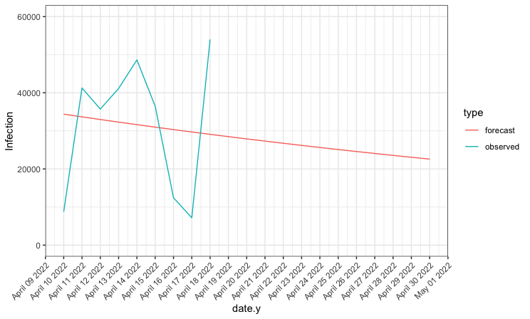
Figure 4: Predicted numbers of new infections compared to actual number of new infections
As seen in the plot above, the true infection data is considerably more variable than our forecasted data, with much lower values associated with weekends. However, if we look at the total infections over the nine days for which we are able to compare our forecast, we see that our model performed well, predicting the total number of infections to within 500 of the observed number.
| Data | Total Infections |
|---|---|
| Forcasted | 285136 |
| Observed | 285621 |
Total Infections for April 10 – 18, 2022
Conclusion
Given the massive scale of the COVID-19 pandemic, traditional SIR models which rely on modeling the probability of infection at very small time intervals or continuous time become computationally infeasible quickly. With thousands of new infections per day in the U.S. alone, it would be impossible to use MCMC methods to estimate the parameters for every new infection and recovery. Our method, which assumes a constant infection rate across each day, effectively utilizes a Bayesian framework to estimate the parameters of the model. Our procedure appears to have done a reasonably good job estimating the infection and recovery rate parameters on both simulated and real data. Though it was not as efficient an algorithm as we desired, it was able to predict with considerable accuracy the total infections over 9 days in the U.S.
Our analysis carries several important limitations. Firstly, researchers are unable to observe recovery times, so knowing the true length of the infectious period for each individual with COVID is impossible, as is verifying the accuracy of predicted recovery counts. Secondly, we are aware that COVID testing and reporting is imperfect, which was true due to a lack of testing early in the pandemic, and is now an issue again due to the common use of home test kits. Thirdly, our model uses highly diffuse prior distributions, which could be improved by consulting with expert epidemiologists. Finally, although we have tried to take into account factors affecting the infection rate such as vaccination rates and mask mandates, our model is likely to still be insufficiently complex to capture the many factors which influence the course of the pandemic.
Continued research modeling the spread of infectious disease is necessary in order to help reduce many of the negative effects of COVID and other disease. We hope that with effective modeling of new infections, governments, institutions, and individuals may be able to implement effective interventions to slow the spread of COVID and reduce the serious health and social consequences of infectious disease.
References
- CDC. Healthcare Workers. https://www.cdc.gov/coronavirus/2019-ncov/hcp/durationisolation.html, February 2020.
- CDC. Omicron variant: What you need to know. May 2022. https://www.cdc.gov/coronavirus/2019ncov/variants/omicron-variant.html.
- Thomas Hale, Noam Angrist, Rafael Goldszmidt, Beatriz Kira, Anna Petherick, Toby Phillips, Samuel Webster, Emily Cameron-Blake, Laura Hallas, Saptarshi Majumdar, and Helen Tatlow. A global panel database of pandemic policies (Oxford COVID-19 Government Response Tracker). Nature Human Behaviour, 5(4):529–538, April 2021. ISSN 2397-3374. doi: 10.1038/s41562-021-01079-8.
- Lucas Rod ́es-Guirao Cameron Appel Charlie Giattino Esteban Ortiz-Ospina Joe Hasell Bobbie Macdonald Diana Beltekian Hannah Ritchie, Edouard Mathieu and Max Roser. Coronavirus pandemic (covid-19). Our World in Data, 2020. https://ourworldindata.org/coronavirus.
- Theodore Kypraios, Peter Neal, and Dennis Prangle. A tutorial introduction to Bayesian inference for stochastic epidemic models using Approximate Bayesian Computation. Mathematical Biosciences,
287:42–53, May 2017. ISSN 0025-5564. doi:10.1016/j.mbs.2016.07.001. - Lili Wang, Yiwang Zhou, Jie He, Bin Zhu, Fei Wang, Lu Tang, Michael Kleinsasser, Daniel Barker,
Marisa C. Eisenberg, and Peter X.K. Song. An epidemiological forecast model and software assessing interventions on the covid-19 epidemic in china. Journal of Data Science, 18(3):409–432, 2021. ISSN 1680-743X. doi: 10.6339/JDS.20200718(3).0003. - Phitchayapak Wintachai and Kiattisak Prathom. Stability analysis of SEIR model related to efficiency of vaccines for COVID-19 situation. Heliyon, 7(4), April 2021. ISSN 2405-8440. doi: 10.1016/j.heliyon.2021.e06812