
The power-law distribution is of the form $f(x) \propto x^{-\alpha}$, where $\alpha$ is called the scaling parameter. It models many natural phenomena like acoustic attenuation, Curie–Von Schweidler law, neuronal avalanches, and others. As $x \to 0$, $f(x)$ diverges out of bounds. Hence, we define $\xmin$ as a lower bound for the support of the distribution function $f(x)$. Using this, the power-law density function can be written as
$$
f(x) = \frac{\alpha-1}{\xmin}\left( \frac{x}{\xmin}\right)^{-\alpha} \ \ \ \ , \ x > \xmin
$$
More generally, the power-law distribution function can be written with an exponential cutoff which is of the form $f(x) \propto x^{-\alpha}e^{-\lambda x}$ , which is again defined for $x > \xmin$. While the estimation of the scaling parameter is quite straightforward with maximum likelihood estimation, or by using a variant of MLE, the estimation of the lower-bound parameter $\xmin$ is quite challenging as it can be overestimated in favor of a high likelihood value. One way to combat this problem is by penalizing the likelihood function for higher $\xmin$, as discussed by Olmez, et.al. Another way to solve this is by using the Bayesian approach, which allows us to impose an appropriate prior on $\xmin$. In this research, I discuss the estimation of the parameters of a power-law distribution with an exponential cutoff in three cases –
- Unknown $\alpha$, and known $\xmin$, $\lambda$
- Unknown $\xmin$ and $\alpha$, and known $\lambda$
- Unknown $\alpha$, $\lambda$, and $\xmin$
Methods
This section discusses the establishment of the Bayesian framework for the distribution, for the three cases involving different priors.
Probability Density Function
As discussed before, the distribution is of the form
$$
f(x) = C x^{-\alpha}e^{-\lambda x} 1(x > \xmin)
$$
It can be easily verified using simple integration: $C = \lambda^{1-\alpha} \ / \ \Gamma(1-\alpha, \lambda \xmin) \ \ $
where,
$\Gamma(1-\alpha, \lambda \xmin)$ is the upper incomplete gamma function defined as,
$$
\Gamma(s,x) = \int_{x}^{\infty} t^{s-1} e^{-t} dt \ \ \ \ , \ x > 0
$$
Bayesian Framework
A general form of the posterior distribution of the parameter space $\boldphi$ conditioned on the given data $\mathcal{D}$ is given by
$$
p(\boldphi \ | \ \mathcal{D}) \propto_{\boldphi} \mathcal{L}(\mathcal{D}, \boldphi) \ p(\boldphi)
$$
where $ \mathcal{D} = { x_1, x_2, \dots, x_n } $
$\mathcal{L}(\mathcal{D}, \boldphi)$ is the likelihood function for the samples given the parameters in the parameter space. In the case of this distribution, the existence of $\xmin$ and the same being a parameter to be estimated (random) adds to the complexity of defining the likelihood function of the data given the parameters $\boldphi = (\alpha, \lambda, \xmin)$.
$$
\begin{aligned}
\mathcal{L}(\mathcal{D}, \boldphi) &= \prod_{x_i > \xmin} f(x_i|\boldphi) \
\end{aligned}
$$
We know that $0 < f(x_i \ | \alpha, \lambda, \xmin) < 1, \ \forall x_i > \xmin$, and hence, for a given $\mathcal{D} = {x_1, x_2, \dots, x_n}$, $\prod_{x_i > \xmin} f(x_i \ | \alpha, \lambda, \xmin)$ decreases monotonically with $\xmin$. To counter this problem, an appropriate prior must be specified for $\xmin$.
$$
\begin{aligned}
\mathcal{L}(\mathcal{D}, \boldphi) &= \prod_{x_i > \xmin} \frac{\lambda^{1-\alpha}} {\Gamma(1-\alpha, \lambda \xmin)} \ x_i^{-\alpha} e^{-\lambda x_i} \ 1(x_i > \xmin) \\
&= \prod_{x_i > \xmin} \frac{\lambda^{1-\alpha}} {\Gamma(1-\alpha, \lambda \xmin)} \ x_i^{-\alpha} e^{-\lambda x_i} \\
&\equiv \prod_{i = 1}^n \left[ \frac{\lambda^{1-\alpha}} {\Gamma(1-\alpha, \lambda \xmin)} \ x_i^{-\alpha} e^{-\lambda x_i} 1(x_i > \xmin) + 1(x_i \le \xmin) \right] \\
\mathcal{L}(\mathcal{D}, \boldphi) &= \prod_{i = 1}^n \left[ \frac{\lambda^{1-\alpha}} {\Gamma(1-\alpha, \lambda \xmin)} \ x_i^{-\alpha} e^{-\lambda x_i} 1(x_i > \xmin) + 1(x_i \le \xmin) \right]\
\end{aligned}
$$
The Bayesian framework can now be written as
$$
p(\boldphi \ | \ \mathcal{D}) \propto_{\boldphi} \prod_{i = 1}^n \left[ \frac{\lambda^{1-\alpha}} {\Gamma(1-\alpha, \lambda \xmin)} \ x_i^{-\alpha} e^{-\lambda x_i} 1(x_i > \xmin) + 1(x_i \le \xmin) \right]\ \ p(\boldphi)
$$
The prior distribution of $\boldphi$ consists of joint prior of $\alpha$, $\lambda$ and $\xmin$.
Jeffrey’s Prior for the Scaling Parameter
Jeffrey’s prior is a non-informative prior. It does not make modeling assumptions of the parameter, and the posterior function thus obtained represents the parameter given the data as best as possible.
Jeffrey’s prior is given by,
$$
\xi^{J}(\phi) \propto_{\phi} \sqrt{I^{F}(\phi)}
$$
Here, $I^{F}(\phi)$ is the Fischer information given by, $$ \begin{aligned} &I^{F}(\phi) = E_{[X|\phi]} \left\{ \frac{\partial}{\partial \phi} \log f(X|\phi) \right\}^2 \\ &\text{or}, \\ &I^{F}(\phi) = – \ E_{[X|\phi]} \left\{ \frac{\partial^2}{\partial \phi^2} \log f(X|\phi) \right\} \end{aligned} $$
To obtain the Jeffrey’s prior for the scaling parameter, we need
$$ \begin{aligned} I^{F}(\alpha) &= – \ E_{[X|\alpha]} \left\{ \frac{\partial^2}{\partial \alpha^2} \log f(X|\alpha) \right\}\\ &= – \ E_{[X|\alpha]} \frac{\partial^2}{\partial \alpha^2} \log \left[ \frac{\lambda^{1-\alpha}} {\Gamma(1-\alpha, \lambda \xmin)} \ x^{-\alpha} e^{-\lambda x} \ 1(x > \xmin) \right] \\ &= – \ E_{[X|\alpha]} \frac{\partial^2}{\partial \alpha^2} \left[ -\alpha \log x – \lambda x +(1-\alpha) \log \lambda + \log1(x>\xmin)- \log \Gamma(1-\alpha, \lambda \xmin) \right] \\ &= – \ E_{[X|\alpha]} \frac{\partial}{\partial \alpha} \left[ -\log x – \log \lambda – \frac{\Gamma_{\alpha}^{\prime} (1-\alpha, \lambda \xmin)}{\Gamma_{\alpha} (1-\alpha, \lambda \xmin)} \right]\\ &= – \ E_{[X|\alpha]} \left[\frac {\gammaone^2 \ – \ [\gammazero \ \gammatwo]}{\gammazero^2} \right]\\ I^{F}(\alpha) &= \frac {[\gammazero \ \gammatwo] \ – \ \gammaone^2 }{\gammazero^2} \end{aligned} $$Here, $\gammaone$ is the first partial derivative of $\gammazero$ with respect to $\alpha$, $\frac{\partial}{\partial \alpha} \gammazero$, and $\gammatwo$ is the second partial derivative of $\gammazero$ with respect to $\alpha$, $\frac{\partial^2}{\partial \alpha^2} \gammazero$. $$ \begin{aligned} \gammaone &= \frac{\partial}{\partial \alpha} \gammazero\\ &= \frac{\partial}{\partial \alpha} \left[ \int_{\lambda \xmin}^{\infty} t^{-\alpha} e^{-t} dt \right]\\ &= \int_{\lambda \xmin}^{\infty} \frac{\partial}{\partial \alpha} (t^{-\alpha}) e^{-t} dt \\ &= \int_{\lambda \xmin}^{\infty} -\alpha t^{-\alpha-1} e^{-t} dt \\ \gammaone &= -\alpha \Gamma(-\alpha, \lambda \xmin)\\ \\ \gammatwo &= \frac{\partial}{\partial \alpha} [-\alpha \Gamma(-\alpha, \lambda \xmin)]\\ &= -\Gamma(-\alpha, \lambda \xmin) – \alpha \int_{\lambda \xmin}^{\infty} (-\alpha-1) t^{-\alpha-2} e^{-t} dt \\ \gammatwo &= \alpha (\alpha + 1) \Gamma(-1-\alpha, \lambda \xmin) -\Gamma(-\alpha, \lambda \xmin) \end{aligned} $$
Hence, our Jeffrey’s prior can be simplified to,
$$ \begin{aligned} \xi^{J}(\phi) &\propto_{\phi} \sqrt{I^{F}(\phi)}\\ &\propto_{\phi} \sqrt{\frac {[\gammazero \ \gammatwo] \ – \ \gammaone^2 }{\gammazero^2} } \\ \xi^{J}(\alpha | \ \lambda, \xmin) &\propto_{\alpha} \sqrt{\frac {[\gammazero \ \{\alpha (\alpha + 1) \Gamma(-1-\alpha, \lambda \xmin) -\Gamma(-\alpha, \lambda \xmin)\}] \ – \ (\alpha \Gamma(-\alpha, \lambda \xmin))^2 }{\gammazero^2}} \end{aligned} $$Priors for the three cases –
- Known $\xmin$, $\lambda$, and unknown $\alpha$: In this case, we can use Jeffrey’s prior on $\alpha$ as it is the only parameter to be estimated. Our posterior is of the form,
$$
p(\boldphi \ | \ \mathcal{D}) \propto_{\boldphi} \prod_{i = 1}^n \left[ \frac{\lambda^{1-\alpha}} {\Gamma(1-\alpha, \lambda \xmin)} \ x_i^{-\alpha} e^{-\lambda x_i} 1(x_i > \xmin) + 1(x_i \le \xmin) \right] \xi^{J}(\alpha)
$$ where $\xi^{J}(\alpha)$ is the Jeffrey’s prior at $\alpha$. - Known $\lambda$, and unknown $\xmin$ and $\alpha$: In this case, we can use a uniform prior on $\alpha$, and an exponential prior with lower and upper bounds on $\xmin$ which would discourage higher values of $\xmin$ on the posterior as discussed before.$$p(\boldphi \ | \ \mathcal{D}) \propto_{\boldphi} \prod_{i = 1}^n \left[ \frac{\lambda^{1-\alpha}} {\Gamma(1-\alpha, \lambda \xmin)} \ x_i^{-\alpha} e^{-\lambda x_i} 1(x_i > \xmin) + 1(x_i \le \xmin) \right] f_{\alpha}(a) \ f_{\xmin}(x)$$ where, $f_{\alpha}(a) \equiv \text{U}(2,3)$ and $f_{\xmin}(x) \propto e^{-10x} \ 1(x>1) 1(x<3)$
- Unknown $\alpha$, $\lambda$, and $\xmin$: In this case, since all three parameters are to be estimated, we use informative priors on each of the parameters. In this case, we use exponential distributions with upper and lower-bound cutoffs on each of them.$$p(\boldphi \ | \ \mathcal{D}) \propto_{\boldphi} \prod_{i = 1}^n \left[ \frac{\lambda^{1-\alpha}} {\Gamma(1-\alpha, \lambda \xmin)} \ x_i^{-\alpha} e^{-\lambda x_i} 1(x_i > \xmin) + 1(x_i \le \xmin) \right] f_{\alpha}(a) \ f_{\lambda}(l) \ f_{\xmin}(x)$$ where, $f_{\alpha}(a) \propto e^{-10a} \ 1(a>2) 1(a<3)$, $f_{\lambda}(l) \propto e^{-10l} \ 1(l>0) 1(l<3)$ and $f_{\xmin}(x) \propto e^{-10x} \ 1(x>1) 1(x<3)$
Simulation
Simulation involves the generation of power-law samples with exponential cutoffs, with true parameters, and the estimation of these parameters. The distribution is complex to sample from using traditional methods like inverse-transform sampling, and hence, we have to use Monte Carlo methods to draw samples. None of our priors are conjugate priors, and we do not have a close-form solution for the posterior. Therefore, to perform parameter estimation, we would need to use Monte Carlo methods.
Generation of the power-law samples with exponential cutoff
Since direct sampling is difficult, we can use Accept-Reject sampling to sample from the distribution. For Accept-Reject sampling, we need to use a covering distribution $g(x)$ for which $M g(x) \ge l(x)$ where $M$ is a scalar, and $l(x) = c \pi(x)$ where $\pi(x)$ is the power-law distribution with exponential cutoff. We can use a traditional power-law distribution (no exponential cut-off) as a covering distribution, as the density of the exponential cutoff declines faster than the traditional power-law distribution.
The probability density function of a traditional power-law distribution is given by,
$$g(x\ | \ x_m,\alpha) = \frac{\alpha-1}{x_m} \left(\frac{x}{x_m}\right)^{-\alpha} \ , \ x>x_m$$
Now we use inverse transform sampling to draw samples from the traditional power-law distribution using uniform random samples.
$$
\begin{aligned}
G(x) &= \int_{-\infty}^x g(x\ | \ x_m,\alpha) \ dx\\
&= \int_{-\infty}^x \frac{\alpha-1}{x_m} \left(\frac{x}{x_m}\right)^{-\alpha} I(x>x_m) \ dx \\
&= \int_{x_m}^x \frac{\alpha-1}{x_m} \left(\frac{x}{x_m}\right)^{-\alpha} \ dx \\
G(x) &= 1- \left( \frac{x}{x_m} \right)^{-\alpha+1}\\
u &= 1- \left( \frac{x}{\xmin} \right)^{-\alpha+1}\\
x &= \xmin(1-u)^{\frac{1}{1-\alpha}}
\end{aligned}
$$
Here, $x$ is a sample from the distribution $g(x|\alpha, \lambda, \xmin)$. It can be shown that,
$$ M = \frac{\lambda^{1-\alpha} \ e^{-\lambda \xmin} \ \xmin} {(\alpha-1) \ \Gamma(1-\alpha, \lambda \xmin) \ \xmin^{\alpha}} $$where, $M$ satisfies the condition, $M g(x) \ge l(x)$
Accept-Reject algorithm:
- Draw $x$ from $g()$
- Compute $$ r = \frac{l(x)}{M g(x)} \ (\le 1) $$
- Draw $f=\text{Bernoulli}(r)$
- if $f = 1$, accept and return $x$
- if $f = 0$, reject $x$
Accept-Rejection sampling to generate Power Law samples with Exponential Cutoff in R
Import the necessary libraries and set a seed
set.seed(84884)
library(expint)
library(remotes)
library(sigmoid)
Set the true-parameters
alpha <- 2.2
lambda <- 0.3
xmin <- 1.1
theta_true <- c(alpha, lambda, xmin)
c <-  lambda^(1-alpha)/(gammainc(1-alpha, lambda*xmin))
Write a function for the PDF of the power-law distribution with an exponential cutoff
fp <- function(x){
  if (x > xmin){
  return(c * ((x^ (-1 * alpha)) * (exp(-1 * lambda * x))))
  }
  else {
    return(0)
  }
}
Write functions to sample from the covering distribution (vanilla power-law)
foo <- function(xmin, alpha){
  u <- runif(1,0,1)
  return(xmin*((1-u)^(1/(1-alpha))))
}
generate <- function(n, xmin, alpha){
  return(as.numeric(replicate(n, foo(xmin, alpha), simplify=FALSE)))
}
getCumulative <- function(x, xmin, alpha){
  return(1-((x/xmin)^(1-alpha)))
}
covering <- function(i){
  return(generate(1, xmin, alpha))
}
Write a function to obtain the PDF of the covering distribution
c_c <- ((alpha-1)/xmin) * (xmin^alpha)
covering_pdf <- function(x){
  if (x > xmin){
    return(((alpha-1)/xmin)*((x/xmin)^(-alpha)))
    }
  else{
    return(0)
  }
}

M <- c*(exp(-lambda*(xmin)))/c_c
I usually like to write a helper function to calculate the Accept-Reject ratio
compute_ratio <- function(u){
  return(fp(u)/(M*covering_pdf(u)))
}
Perform Accept-Reject sampling
samples <- list()
for (i in 1:500){
sample <- covering()
r <- compute_ratio(sample)
result <- rbinom(1,1,prob=r)
if (result == 1){
samples <- c(samples, sample)
}
}
samplesPL <- as.numeric(samples)
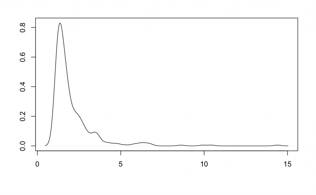
length(samplesPL)We can now plot the density of the power-law samples obtained from the Accept-Reject sampling method
plot(density(samplesPL), xlab = "x", ylab = "Frequency", main="Density")
Bayesian inference on the parameters
Bayesian inference using Monte Carlo methods involves sampling from the posterior to find the parameter that gives the highest value on the posterior (mode of the posterior distribution). Since in case 2 and case 3, we need to estimate more than one parameter, our sampling from the posterior involves drawing random vectors from the posterior. In this case, we use the Metropolis-Hasting algorithm for drawing samples from the posterior. Given a proposal distribution $q(\boldsymbol{\phi_i} | \boldsymbol{\phi_{i-1}})$ and the likelihood function $\mathcal{L}(\mathcal{D}, \boldphi)$.
- Start with $\boldsymbol{\phi_0}$
- For $i=1, 2, \dots n$:
- Draw $\boldsymbol{\phi^*}$ from $q(\boldsymbol{\phi_{i-1}})$
- Compute $a = \frac{\mathcal{L}(\mathcal{D}, \boldsymbol{\phi^*}) q(\boldsymbol{\phi_{i-1}} | \boldsymbol{\phi^*})}{\mathcal{L}(\mathcal{D}, \boldsymbol{\phi_{i-1}}) q(\boldsymbol{\phi^*} | \boldsymbol{\phi_{i-1}})}$
- if $a > 1$, accept $\boldsymbol{\phi^*}$, $\boldsymbol{\phi_i} = \boldsymbol{\phi^*}$
- if $0 < a < 1$, accept $\boldsymbol{\phi^*}$, $\boldsymbol{\phi_i} = \boldsymbol{\phi^*}$ with probability $a$
Our proposal distributions, like prior distributions, vary with each case.
- Case 1: $q(x | \boldsymbol{\phi_{i-1}}) = \boldsymbol{\phi_{i-1}} e^{\boldsymbol{\phi_{i-1}} \ x} \ 1(1>0)$
- Case 2: $\boldsymbol{q}(\boldsymbol{x} | \boldsymbol{\phi_{i-1}}) = \begin{bmatrix} \boldsymbol{\phi_{i-1}}^{[1]} e^{\boldsymbol{\phi_{i-1}}^{[1]} \ x_1} \ 1(x_1>0) \\ \boldsymbol{\phi_{i-1}}^{[2]} e^{\boldsymbol{\phi_{i-1}}^{[2]} \ x_2} \ 1(x_2>0) \\ \end{bmatrix} $
- Case 3: $ \boldsymbol{q}(\boldsymbol{x} | \boldsymbol{\phi_{i-1}})= \begin{bmatrix} \boldsymbol{\phi_{i-1}}^{[1]} e^{\boldsymbol{\phi_{i-1}}^{[1]} \ x_1} \ 1(x_1>0) \\ \boldsymbol{\phi_{i-1}}^{[2]} e^{\boldsymbol{\phi_{i-1}}^{[2]} \ x_2} \ 1(x_2>0) \\ \boldsymbol{\phi_{i-1}}^{[3]} e^{\boldsymbol{\phi_{i-1}}^{[3]} \ x_3} \ 1(x_3>0)\\ \end{bmatrix} $
Case 1 :
- Alpha – Jeffrey’s prior
- Lambda – known
- xmin – known
lambda <- theta_true[2]
xmin <- theta_true[3]
Gamma function
G <- function(alpha){
  suppressWarnings(gammainc(1-alpha, lambda*xmin))
}
The first derivative of the Gamma function
Gp1 <- function(alpha){
  -1 * alpha * suppressWarnings(gammainc(-1*alpha, lambda*xmin))
}
The second derivative of the Gamma function
Gp2 <- function(alpha){
  (alpha*(alpha+1)*suppressWarnings(gammainc(-1-alpha, lambda*xmin))) - suppressWarnings(gammainc(-1*alpha, lambda*xmin))
}
prior_alpha <- function(alpha){
j <- ((G(alpha)*Gp2(alpha))-(Gp1(alpha)^2))/(G(alpha)^2)
if (is.na(j)){
return(0)
}
if (j < 0){
j <- j*-1
} else{
return(sqrt(j))
}
}pllikelihood <- function(x, alpha){
if (x > xmin){
return(((x^(-alpha)) * exp(-lambda * x) * (lambda^(1 - alpha)))/suppressWarnings(gammainc(1-alpha, lambda * xmin)))
}
else {
return(1)
}
}loglikelihood <- function(data, alpha){
lik <- lapply(data, pllikelihood, alpha=alpha)
blee <- lapply(lik, log)
return(sum(as.numeric(blee)))
}Posterior distribution known up to a constant
logpostfunc <- function(data, alpha){
  alpha <- as.numeric(alpha)
  return(loglikelihood(data, alpha)+log(prior_alpha(alpha)))
}
Proposal distribution
proposal <- function(given){
  k <- as.numeric(given)
  return(rexp(1, k))
}
proposal_pdf <- function(this, given){
return(dexp(as.numeric(this), as.numeric(given)))
}Metropolis-Hasting for Bayesian Inference
reps <- 100
acc <- list()
params <- list()
pb = txtProgressBar(min = 1, max = reps, initial = 1)
for (v in 1:reps){
  nit <- 100
  accepted <- 0
  theta <- list()
  theta[1] <- proposal(2.1)
  for(i in 2:nit){
    theta_star <- proposal(theta[i-1])
    a = (logpostfunc(samplesPL, theta_star) + log(proposal_pdf(theta[i-1],
                    theta_star)))-logpostfunc(samplesPL,theta[i-1]) - log(proposal_pdf(theta_star,theta[i-1]))
    a <- exp(a)
    if (is.nan(a)){
      theta[i] <-  theta[i-1]
    } else if (a > 1){
      theta[i] <-  theta_star
      accepted <- accepted+1
    } else{
      r = rbinom(1,1,a)
      if (r == 1){
        theta[i] <-  theta_star
        accepted <- accepted+1
      } else{
        theta[i] <-  theta[i-1]
      }
    }
  }
  acc[v] <- accepted/nit
  post_pdf <- lapply(theta, logpostfunc, data=samplesPL)
  theta_selected <- theta[which.max(post_pdf)]
  params[v] <- theta_selected
  setTxtProgressBar(pb,v)
}
params <- as.numeric(params)
plot(d, xlab = "alpha", ylab = "Density", main = "Density of alpha on the posterior")
abline(v=d$x[i], col="blue")
abline(v=alpha, col="red")mean(params)The MCMC algorithm implementation for the rest of the cases is a bit more complex as it involves random walks in higher dimensions. It can be found on my GitHub page.
Results
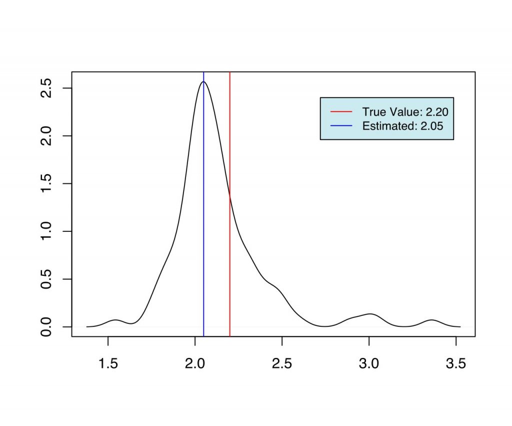
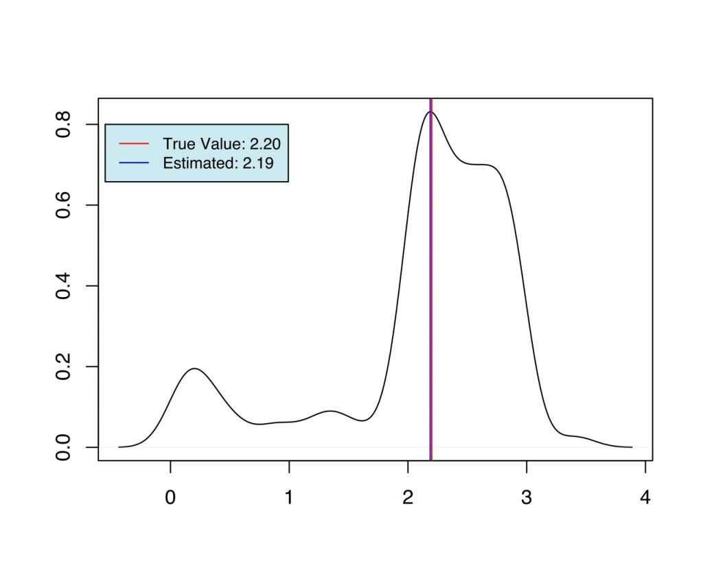
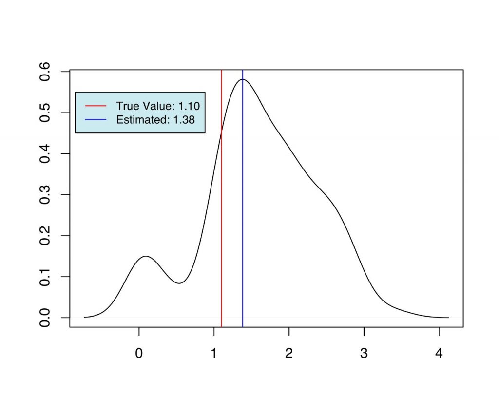
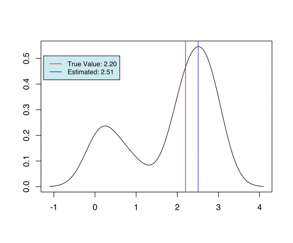
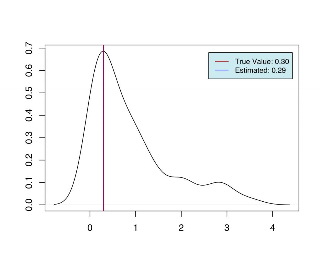
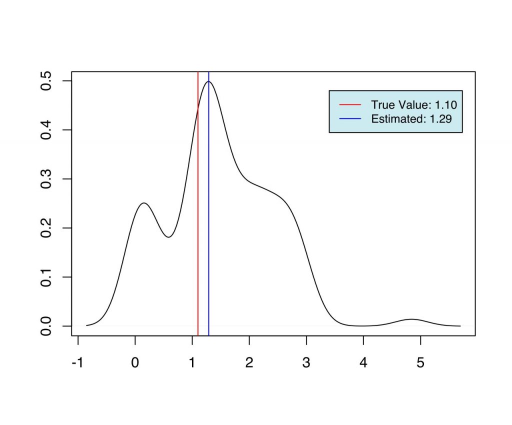
The simulation discussed above is implemented in R. For each case, the same samples are used, which are drawn from the distribution with the true parameters using Accept-Reject sampling. We generate 355 samples from the distribution with the true parameters, $\alpha=2.2$, $\lambda=0.3$, and $\xmin=1.1$, and use the same for inference in the three cases discussed above. In each of the three cases, the Metropolis-Hasting algorithm was used to draw 1000 samples ${\boldsymbol{\phi}^{[1]}, \boldsymbol{\phi}^{[2]} \dots \boldsymbol{\phi}^{[1000]}}$ from the posterior, and $\hat{\boldsymbol{\phi}} = \text{argmax}_{\boldsymbol{\phi}} \ p(\boldphi \ | \ \mathcal{D})$ is calculated, where, $\mathcal{D}$ is the sample generated from the distribution with known true parameters. This is repeated 100 times to calculate the estimate ($\hat{\boldsymbol{\phi}}$) at each iteration.
As we can see from Fig (1-6), we have the set of estimates for the parameters in each case, which are very close to the true value used during the simulation. When priors are more informative (case 2 and case 3), and when the number of estimable parameters is lower (case 1 and 2) we have better estimates of the parameters.
| Case | Parameter | True | Estimated |
| 1 | $\alpha$ | 2.2 | 2.05 |
| 2 | $\alpha$ | 2.2 | 2.19 |
| 2 | $\xmin$ | 1.1 | 1.38 |
| 3 | $\alpha$ | 2.2 | 2.51 |
| 3 | $\lambda$ | 0.3 | 0.29 |
| 3 | $\xmin$ | 1.1 | 1.29 |
Conclusion
In this research, we used MCMC for Bayesian parameter estimation from a power-law distribution with an exponential cutoff. First, we implemented an Accept-Reject method to sample from the distribution for later inference. Then, we derived Jeffrey’s prior for one of the cases and used the Metropolis-Hasting algorithm to sample from the prior. For the proposal function, we derived the inverse transform sampling function for the traditional power-law distribution. Parameters were then estimated from the posterior samples by finding the mode.
In disciplines where we encounter power-law distributions in empirical data, having prior knowledge of the parameters and their bounds can significantly improve Bayesian estimations as observed. Even though this method can be used for estimation, for case 3, efficiency was as low as 15%. For inference on higher parameter dimensions, Hamiltonian Monte-Carlo can be used to yield higher efficiency.
References
- A. Clauset, C. R. Shalizi, and M. E. J. Newman, “Power-Law Distributions in Empirical Data,” SIAM Review, vol. 51, no. 4. Society for Industrial & Applied Mathematics (SIAM), pp. 661–703, Nov. 04, 2009. doi: 10.1137/070710111
- Z. Zhu and R. A. Marcus, “A Maximum Likelihood Method for Power-law Distributions That Does Not Break Down When the Slope Is Close to Unity,” The Journal of Physical Chemistry C, vol. 116, no. 27. American Chemical Society (ACS), pp. 14690–14693, Jun. 20, 2012. doi: 10.1021/jp303697j
- F. Olmez, P. R. Kramer, J. Fricks, D. R. Schmidt, and J. Best, “Penalized KS method to fit data sets with power-law distribution over a bounded subinterval,” Journal of Statistical Computation and Simulation, vol. 91, no. 8. Informa UK Limited, pp. 1524–1563, Jan. 14, 2021. doi: 10.1080/00949655.2020.1861281
- B. Nettasinghe and V. Krishnamurthy, “Maximum Likelihood Estimation of Power-law Degree Distributions via Friendship Paradox-based Sampling,” ACM Transactions on Knowledge Discovery from Data, vol. 15, no. 6. Association for Computing Machinery (ACM), pp. 1–28, May 19, 2021. doi: 10.1145/3451166
- Harney, Hanns L. Bayesian inference : parameter estimation and decisions. Berlin New York: Springer, 2003
- F. Pennini and A. Plastino, “Power-law distributions and Fisher’s information measure,” Physica A: Statistical Mechanics and its Applications, vol. 334, no. 1–2. Elsevier BV, pp. 132–138, Mar. 2004. doi: 10.1016/j.physa.2003.10.076
- Liu, Jun S. Monte Carlo strategies in scientific computing. New York: Springer, 2008
- Casella, George, and Roger L. Berger. Statistical inference. Australia Pacific Grove, CA: Thomson Learning, 2002
- Michael I. Jordan Jeffreys Priors and Reference Priors. Berkeley, CA: Bayesian Modeling and Inference February 17, 2010
- Michael Betancourt: “A Conceptual Introduction to Hamiltonian Monte Carlo”, 2017; [http://arxiv.org/abs/1701.02434 arXiv:1701.02434